Prune and Tune Ensembles: Low-Cost Ensemble Learning With Sparse Independent Subnetworks

(AAAI 2022)

 

https://github.com/tjwhitaker/prune-and-tune-ensembles

GitHub - tjwhitaker/prune-and-tune-ensembles

 

 

Abstract

 

Deeplearning의 ensemble은 효과적이고 좋지만, computational cost가 비싸다는 단점이 있다.

그래서, 이 논문에서는 빠르고 작은 cost로 scratch부터 다양한 모델을 학습할 필요가 없는 ensemble방법을 소개한다.

 

일단 single parent network를 하나 학습하고 child network는 parent를 clone해서 생성한다.

그리고 각 child를 pruning을 통해서 ensemble member로 만든다.

그 후에 각 child를 작은 epoch로 학습하면, scratch부터 학습한 것보다 더욱 빠르게 수렴시킬 수 있다.

 

다양성을 높이기 위해, anti-random pruning + one-cycle tuning 등 다양한 방법을 시도해봤다.

결과적으로 기존 ensemble보다 training cost적인 측면에서 장점이 많다.

 

---

Introduction

 

Ensemble Learning은 각 모델의 결과를 조합하여 unseen data에 대한 generalization을 간단하게 하며, 많은 competitions에서 높은 점수를 기록했지만, 데이터셋과 network가 커짐에 따라, 기존 ensemble 방법은 사용하기 힘들었다.

 

networks를 ensemble할때 큰 computational cost를 줄이는 여러 방법들이 소개됐다.

1. pesudo-ensembles
2. temporal ensembles
3. evolutionary ensembles,
   • (scratch부터 학습할 필요가 없도록 구성원간의 traning정보나 network구조를 공유하는 등)

하지만, cost를 줄이긴 했으나, 종종 potential ensemble size, member diversity, convergence efficiency에 제약을 주면서, 성능이슈가 있었다.

 

이 논문에서는 ensemble size M을 다이나믹하게 생성할 수 있는 향상된 low-cost method를 소개한다.

 

scratch부터 각각 독립적으로 학습하는 것이 아닌, 하나의 큰 부모 network만 학습하여 시작할 수 있다.

1. 학습한 부모 네트워크를 M번 clone하고, random prune하여 M개의 child network를 생성한다.
2. 각 child에 대해 아주 작은 epoch로 fine tune을 진행한다.
   • child를 생성하여 ensemble diversity를 극대화할때, anti-random pruning과 one-cycle tuning을 사용했다

논문의 연구에 따르면, child network의 loss landscape는 같은 부모 네트워크에게 받았음에도, anti-random pruning과 one-cycle tuning으로 local optima에 수렴이 보장됨을 확인했다.

다양한 하이퍼파라미터로 실험한 결과, low-cost ensemble algorithms보다 성능이 향상된 SOTA를 달성했다.

 

---

 

Prune and Tune Ensembles

 

Parent Network

 

그 어떠한 학습 조건도 필요없다.

Any architecture, o|ptimzation methods, normalization, weight decay, dropout, etc.

 

Creating the Ensemble Members

 

부모 network를 clone하고 pruning하여 ensemble member를 만든다.

현재 pruning methods는 대부분 중요계수나 gradient등을 보고, deterministically best params를 선택한다.

위의 방법이, 더 작고 정확도가 높은 single network를 만들 수 있지만, diversity를 위해서는 random pruning이 더 좋다고 가정했다.

 

Anti-Random Pruning

 

기존 random pruning은 children사이에 일정부분을 공유하게 될 가능성이 있다.

이를 부모의 params는 유지하되, 기존 child와 최대한 다르도록 child를 생성해주는 Anti-Random Pruning을 제안했다.

 

pruned connections를 표현하기 위해, binary bit mask를 사용한다.

bit mask끼리 Cartesian distance가 최대가 되도록 구성했다.

$CD(A, B) = \sqrt{| a_{1} - b_{1} | + \dots + |a_{N} - b_{N} |}$

 

모든 ensemble members $ \{ C_{1}, \dots, C_{N} \} $ 의 total distance $TD$ 가 최대가 되는 것을 원하므로 $TD$ 값은 아래와 같다.

$TD = \sum_{i=1}^{N} \sum_{j=1}^{N} CD(C_{i}, C_{j}) $

 

이 과정에서 distance가 최대가 되도록 ensemble을 만드는 것은, 모든 ensemble member에 대한 광범위한 search가 필요한데,

high-dimension network에 대해서는 광범위한 seach가 불가능하다.

 

대신, mask와 partitioning을 통해 distant networks를 만드는 방법으로 해결할 수 있다.

bit string $M$ 에 대해서, 가장 다른 bit string $M'$은 $M' = 1-M$ 이다. 

 

Parent network $W_{p}$에 대해, 50%의 sparsity로 random bit mask를 $n$개를 만든다.

$M = \{ m_{0}, m_{1}, \dots, m_{n} \}$

$C_{1} = W_{p} \circ M$ and $C_{2} = W_{p} \circ M' $

이를 $N$번 반복하면,  50% sparsity를 갖는 $2N$사이즈의 ensemble member를 만들 수 있다.

큰 network에 대해서 적용할때, $N$개의 ensemble을 만든다고 하면, 각 child는 $\frac{1}{N}$사이즈의 params를 갖게 된다.

 

Tuning The Ensemble Members

 

이미 parent network가 잘 학습되었기 때문에, child network는 몇번의 epoch만으로도 수렴할 수 있다.

각 child network의 topology가 다르기 때문에, model들은 다른 곳으로 수렴한다.

 

Bagging

 

각 child network는 무작위로 선택된 90%의 training data를 사용함으로써, diversity를 증가시켰다.

 

Traditional Fine Tuning

 

부모 network에서 사용한 최종적인 lr을 사용하여, 90% training subset을 추가 학습했다.

 

One-Cycle Tuning

 

child networks의 diversity를 증가시키기 위해, one-cycle learning rate schedule을 사용했다.

one-cycle learning rate schedule은 3가지 단계로 구성되어있다.

1. (warm up) 작은 learning rate부터 학습하며 점차 키워간다.
2. (cool down) 큰 learning rate부터 init learning rate보다 몇 배는 작게 줄여간다.
3. (annihilation) learning rate를 0로 만든다.

large lr은 부모 network로 부터 더욱 크게 벗어나게 도와준다. (training budgets이 클수록 좋다.)

논문에서는 위의 3단계를 2단계 cosine annealing로 줄여서 사용한다.

 

1. (warm up) 10%의 traning budget으로 빠르게 낮은 lr $(\eta_{min})$ 부터 main training의 높은 lr$(\eta_{max})$ 까지 키워간다.
2. (cool down) lr을 $1e-7$보다 작게 줄인다.

lr은 batch마다 업데이트한다. ($T_{cur}$은 현재 iteration, $T_{max}$는 total iteration을 말한다.)

$\eta_{t} = \eta_{min} + \frac{1}{2} (\eta_{max} - \eta_{min}) (1 + cos(\frac{T_{cur}}{T_{max}}\pi))$

 

Making Predictions

 

대부분의 ensemble에서 사용하는 방법은 majority vote와 weighted model averaging이다.

이 논문에서는 model averaging을 사용했다.

 

더 좋은 normalization을 위해, member들의 output에 softmax를 취한 값을 average하여 사용했다.

$y_{e} = argmax(\frac{1}{S}\sum^{S}_{i=1}\sigma(f_{i}(x)))$

$y_{e}$는 ensemble prediction, $S$는 ensemble member size, $\sigma$는 softmax function을 말한다.

 

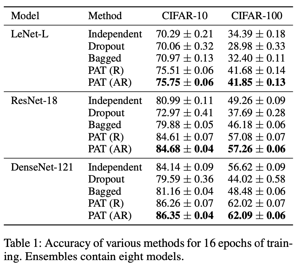
Comparisons for Small Traning Budgets (Prune and Tune)

• only training 16epoch. 
• 8children using anti-random pruning
• 4pairs of network / anti-networks each with 50% sparsity.
• fine tune each child for only 1 epoch.
• ADAM optimizer
• fixed lr 0.001 

Comparisons for Large Training Budgets 

• (Prune and Tune)
  • 200epoch with WideResNet-28-10
  • Stochastic Gradient Decent with Nesterov momentum $\mu = 0.9$, weight decay $\gamma = 0.0005$
  • training 128batchsize, random crop, random horizontal flip, mean std scaling
  • parent
    • step-wise decay schedule.
      • 0.1 (~50%)
      • decay linearly 0.001 (50 ~90%)
      • 0.001 (90% ~ 100%)
• (Prune and Tune Ensembles)
  
  • train a single parent network for 140 epochs.
  • 6 children are created with anti-random pruning (50% sparsity)
  • tune one-cycle learning rate for 10 epochs.
    • 0.001 to 0.1 at 1epoch.
    • decay to $1e-7$ using cosine annealing for final 9 epochs.

 

---

Result

 

Conclusion

 

The Prune and Tune Ensemble algorithm is flexible and enables the creation of diverse and accurate ensembles at a significantly reduced computational cost.

We do this by 1) training a single large parent network, 2) creating child networks by copying the parent and significantly pruning them using random or anti-random sampling strategies, and 3) fine tuning each of the child networks for a small number of training epochs.

We hope to fur- ther explore larger scale benchmarks, anti-random pruning methodologies and applications to new problem domains in future work.